
If you work with data in Excel, you might often feel confused when the data becomes too large. It becomes hard to understand patterns, totals, or comparisons.
This is where a pivot table in Excel helps you.
A pivot table allows you to summarize, analyze, and organize large amounts of data in just a few clicks. You don’t need complex formulas. Instead, you can quickly turn raw data into useful insights.
Let’s understand everything step by step.
What is a Pivot Table in Excel?
A pivot table in Excel is a tool that helps you summarize large data sets. It allows you to:
- Group data
- Calculate totals
- Compare values
- Create reports easily
For example, if you have sales data, you can quickly find:
- Total sales by product
- Sales by region
- Monthly performance
So, instead of scrolling through thousands of rows, you get a clean summary.
Why Should You Use a Pivot Table?
You might wonder, why not just use formulas?
Here’s why pivot tables are better:
- They save time
- You don’t need advanced Excel skills
- You can change the report instantly
- They reduce manual errors
In short, they make data analysis simple and fast.
How to Create a Pivot Table in Excel (Step-by-Step)
Now, let’s see how you can create a pivot table.
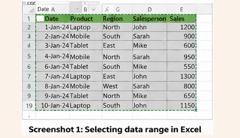
Step 1: Select Your Data
First, open your Excel file and select the data range.
Make sure:
- Your data has headers
- There are no empty rows or columns
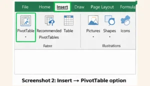
Step 2: Go to the Insert Tab
Now, go to the top menu and click on Insert.
Then click on PivotTable.
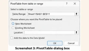
Step 3: Choose Table Location
A pop-up will appear.
Here you can:
- Select your data range (already selected)
- Choose where to place the pivot table
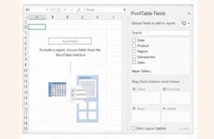
Step 4: Create Your Pivot Table
Now you will see a blank pivot table and a field list on the right side.
You can drag fields into:
- Rows
- Columns
- Values
- Filters
Example of Pivot Table in Excel
Let’s understand with a simple example.
Example: Sales Data
Suppose you have data like:
- Product Name
- Region
- Sales Amount
Now you want to see the total sales by product.
Drag:
- Product → Rows
- Sales → Values
Excel will automatically calculate totals.
How to Use Pivot Table in Excel Effectively
Now that you know how to create it, let’s learn how to use it properly.
1. Filter Data Easily
You can add filters to focus on specific data.
👉 Drag any field into the Filters area.
This helps you view only selected data.
2. Change Value Calculation
By default, Excel shows Sum.
But you can also show:
- Count
- Average
- Max / Min
👉 Click on value field → Value Field Settings
3. Sort Data
You can sort data from highest to lowest.
👉 Right-click on values → Sort
This helps you quickly find top-performing items.
4. Refresh Pivot Table
If your data changes, you need to update the pivot table.
👉 Right-click → Refresh
Common Mistakes to Avoid
While using pivot tables, many beginners make small mistakes.
Avoid these:
- Not selecting complete data
- Missing headers
- Forgetting to refresh data
- Using messy data
Keeping your data clean will give better results.
Pro Tips for Better Results
Here are some useful tips:
- Always use clean and structured data
- Use tables (Ctrl + T) before creating pivot tables
- Try different layouts to understand data better
- Use slicers for better filtering
These small tricks can improve your workflow a lot.
Bottom Line
A pivot table in Excel is one of the most powerful tools for data analysis. It helps you turn complex data into simple insights without using formulas.
Once you start using pivot tables, you will save a lot of time and effort. Also, your reports will become more clear and professional.
So, start practicing today and explore different ways to use pivot tables in your daily work.
FAQs
1. What is a pivot table in Excel used for?
It is used to summarize, analyze, and organize large data sets quickly.
2. Is the pivot table difficult to learn?
No, it is very easy. You can learn it with basic practice.
3. Can I update a pivot table?
Yes, you can refresh it anytime when your data changes.
Read Also –
1- Excel Shortcut Keys
2- Average Formula in Excel